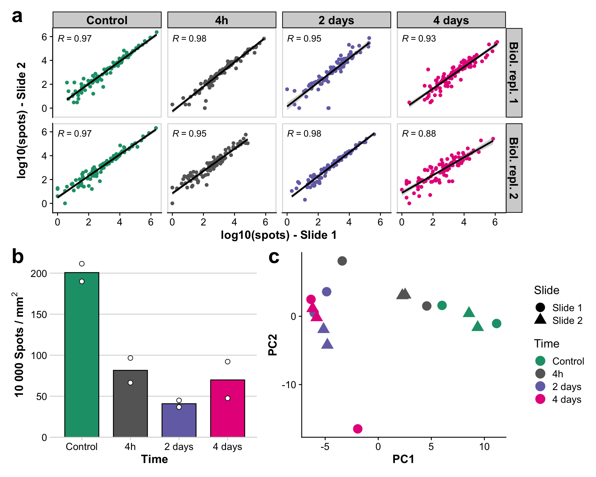
Supplementary Figure 2 : Quality control (QC) of Molecular Cartography data
Florian Wuennemann
Last updated: 2024-03-21
Checks: 7 0
Knit directory: mi_spatialomics/
This reproducible R Markdown analysis was created with workflowr (version 1.7.1). The Checks tab describes the reproducibility checks that were applied when the results were created. The Past versions tab lists the development history.
Great! Since the R Markdown file has been committed to the Git repository, you know the exact version of the code that produced these results.
Great job! The global environment was empty. Objects defined in the global environment can affect the analysis in your R Markdown file in unknown ways. For reproduciblity it’s best to always run the code in an empty environment.
The command set.seed(20230612) was run prior to running
the code in the R Markdown file. Setting a seed ensures that any results
that rely on randomness, e.g. subsampling or permutations, are
reproducible.
Great job! Recording the operating system, R version, and package versions is critical for reproducibility.
Nice! There were no cached chunks for this analysis, so you can be confident that you successfully produced the results during this run.
Great job! Using relative paths to the files within your workflowr project makes it easier to run your code on other machines.
Great! You are using Git for version control. Tracking code development and connecting the code version to the results is critical for reproducibility.
The results in this page were generated with repository version e6213a5. See the Past versions tab to see a history of the changes made to the R Markdown and HTML files.
Note that you need to be careful to ensure that all relevant files for
the analysis have been committed to Git prior to generating the results
(you can use wflow_publish or
wflow_git_commit). workflowr only checks the R Markdown
file, but you know if there are other scripts or data files that it
depends on. Below is the status of the Git repository when the results
were generated:
Ignored files:
    Ignored:    .DS_Store
    Ignored:    .Rproj.user/
    Ignored:    analysis/.DS_Store
    Ignored:    analysis/deprecated/.DS_Store
    Ignored:    analysis/molecular_cartography_python/.DS_Store
    Ignored:    analysis/seqIF_python/.DS_Store
    Ignored:    analysis/seqIF_python/pixie/.DS_Store
    Ignored:    analysis/seqIF_python/pixie/cell_clustering/
    Ignored:    annotations/.DS_Store
    Ignored:    annotations/SeqIF/.DS_Store
    Ignored:    annotations/molkart/.DS_Store
    Ignored:    annotations/molkart/Figure1_regions/.DS_Store
    Ignored:    annotations/molkart/Supplementary_Figure4_regions/.DS_Store
    Ignored:    data/.DS_Store
    Ignored:    data/140623.calcagno_et_al.seurat_object.rds
    Ignored:    data/Calcagno2022_int_logNorm_annot.h5Seurat
    Ignored:    data/IC_03_IF_CCR2_CD68 cell numbers.xlsx
    Ignored:    data/Traditional_IF_absolute_cell_counts.csv
    Ignored:    data/Traditional_IF_relative_cell_counts.csv
    Ignored:    data/pixie.cell_table_size_normalized_cell_labels.csv
    Ignored:    data/results_cts_100.sqm
    Ignored:    data/seqIF_regions_annotations/
    Ignored:    data/seurat/
    Ignored:    output/.DS_Store
    Ignored:    output/mol_cart.harmony_object.h5Seurat
    Ignored:    output/molkart/
    Ignored:    output/proteomics/
    Ignored:    output/results_cts.lowres.125.sqm
    Ignored:    output/seqIF/
    Ignored:    pipeline_configs/.DS_Store
    Ignored:    plots/
    Ignored:    references/.DS_Store
    Ignored:    renv/.DS_Store
    Ignored:    renv/library/
    Ignored:    renv/staging/

Untracked files:
    Untracked:  analysis/deprecated/figures.supplementary_figureX.Rmd
    Untracked:  analysis/deprecated/figures.supplementary_figure_X.MistyR.Rmd

Unstaged changes:
    Deleted:    analysis/figures.supplementary_figureX.Rmd
    Deleted:    analysis/figures.supplementary_figure_X.MistyR.Rmd
    Deleted:    analysis/figures.supplementary_figure_X.proteomics_qc.Rmd
    Deleted:    figures/Figure_5.eps
    Deleted:    figures/Figure_5.pdf
    Deleted:    figures/Figure_5.png
    Deleted:    figures/Figure_5.svg
    Deleted:    figures/Supplementary_Figure_1_Molecular_Cartography_ROIs.png
    Deleted:    figures/Supplementary_figure_5.segmentation_metrics.poster.eps
    Modified:   figures/Supplementary_figure_X.proteomics.eps
    Modified:   figures/Supplementary_figure_X.proteomics.png
    Deleted:    results_cts.lowres.125.sqm
Note that any generated files, e.g. HTML, png, CSS, etc., are not included in this status report because it is ok for generated content to have uncommitted changes.
These are the previous versions of the repository in which changes were
made to the R Markdown
(analysis/figures.supplementary_figure_2.QC_spots.Rmd) and
HTML (docs/figures.supplementary_figure_2.QC_spots.html)
files. If you’ve configured a remote Git repository (see
?wflow_git_remote), click on the hyperlinks in the table
below to view the files as they were in that past version.
| File | Version | Author | Date | Message |
|---|---|---|---|---|
| Rmd | 56559c7 | FloWuenne | 2024-03-21 | Cleaned up repository. |
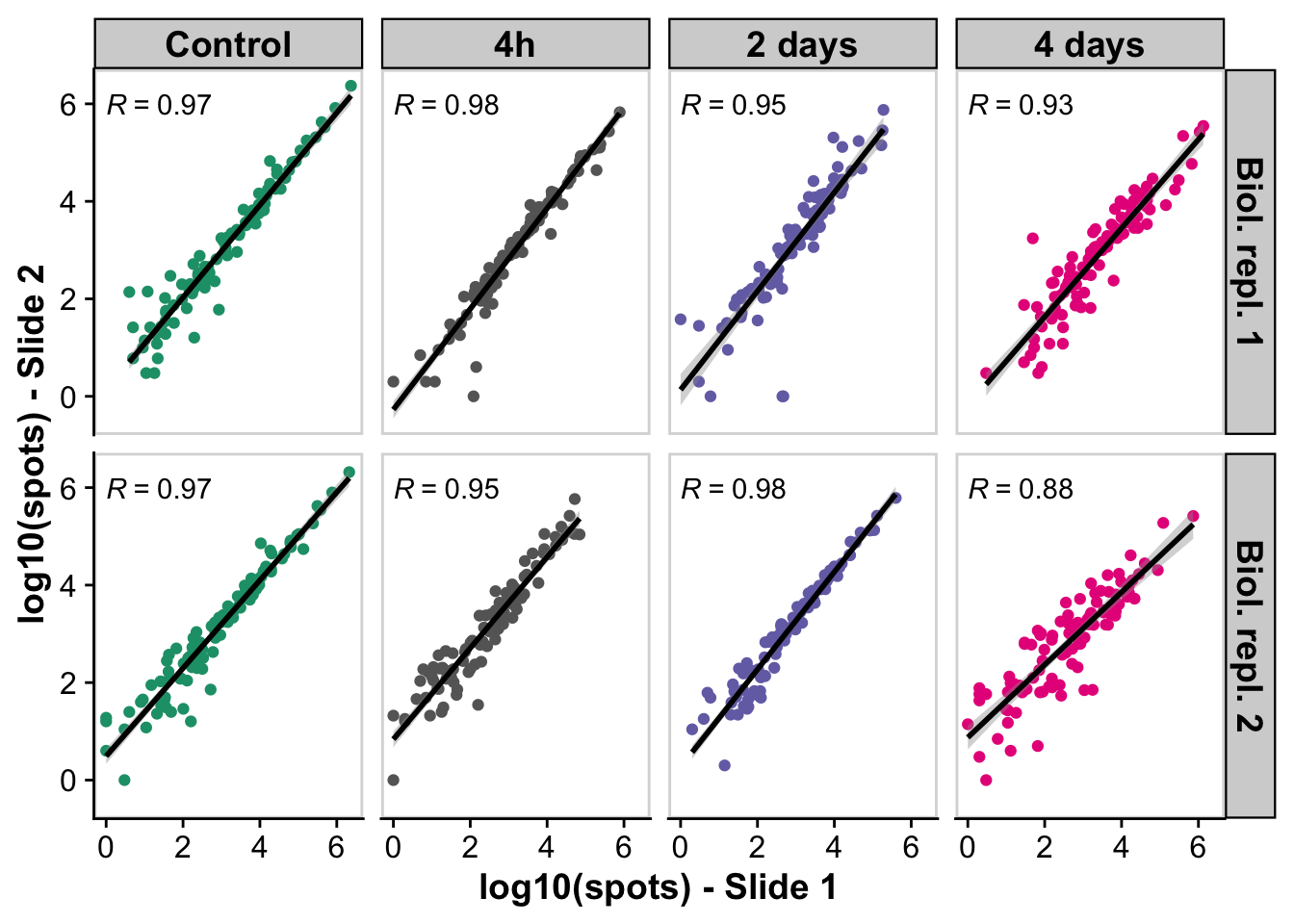
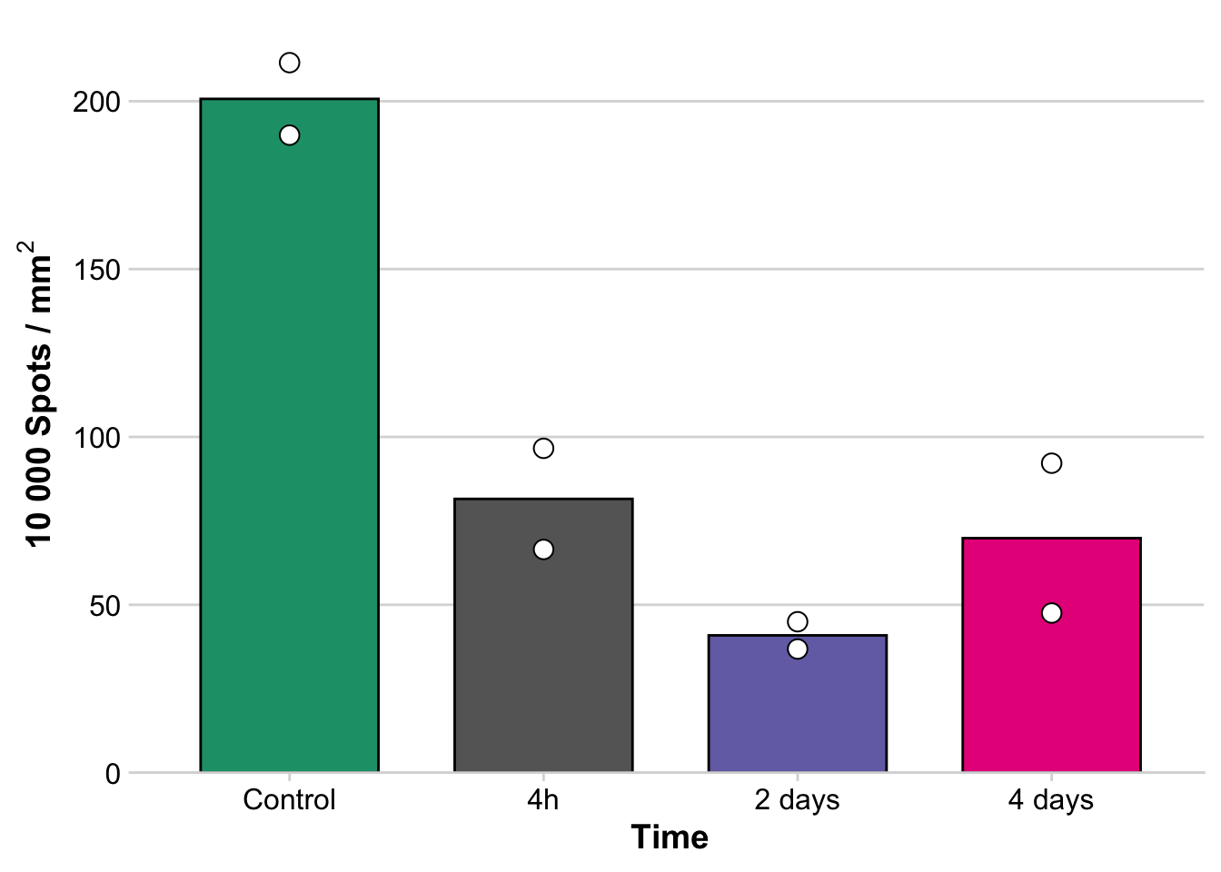
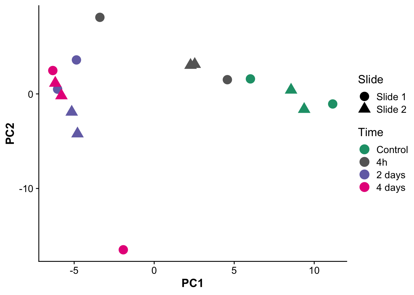
Supplementary Figure 2 - Quality control (QC) of Molecular Cartography data
The data used in this plot was calculated using the following scripts:
A) Correlation between technical replicates
merge_tx_sums <- vroom("./output/molkart/tx_abundances_per_slide.tsv")Rows: 799 Columns: 5
── Column specification ────────────────────────────────────────────────────────
Delimiter: "\t"
chr (3): gene, sample_ID, time
dbl (2): total_tx_rep1, total_tx_rep2
ℹ Use `spec()` to retrieve the full column specification for this data.
ℹ Specify the column types or set `show_col_types = FALSE` to quiet this message.merge_tx_sums_split <- merge_tx_sums %>%
separate(sample_ID, into = c("string","time","replicate"))
# Replace replicate by slide ID
merge_tx_sums_split$replicate <- gsub("r1","Biol. repl. 1",merge_tx_sums_split$replicate)
merge_tx_sums_split$replicate <- gsub("r2","Biol. repl. 2",merge_tx_sums_split$replicate)
merge_tx_sums_split$time <- gsub("control","Control",merge_tx_sums_split$time)
merge_tx_sums_split$time <- gsub("2d","2 days",merge_tx_sums_split$time)
merge_tx_sums_split$time <- gsub("4d","4 days",merge_tx_sums_split$time)
# Set order of time
merge_tx_sums_split$time <- factor(merge_tx_sums_split$time,
levels = c("Control","4h","2 days","4 days"))
tx_correlation_plot <- ggplot(merge_tx_sums_split,aes(log10(total_tx_rep1),log10(total_tx_rep2))) +
geom_point(aes(color = time)) +
geom_smooth(method = "lm", color = "black") +
labs(x = "log10(spots) - Slide 1",
y = "log10(spots) - Slide 2") +
stat_cor(aes(label = ..r.label..), method = "spearman") +
facet_grid(replicate ~ time) +
#scale_color_brewer(palette = "Dark2") +
scale_color_manual(values = time_palette) +
theme(strip.text = element_text(face = "bold", color = "black", size = 14),
strip.background = element_rect(fill = "lightgrey", linetype = "solid",
color = "black", linewidth = 0.8),
axis.title = element_text(face="bold"),
legend.position = "none"
) +
panel_border()
tx_correlation_plotWarning: The dot-dot notation (`..r.label..`) was deprecated in ggplot2 3.4.0.
ℹ Please use `after_stat(r.label)` instead.
This warning is displayed once every 8 hours.
Call `lifecycle::last_lifecycle_warnings()` to see where this warning was
generated.`geom_smooth()` using formula = 'y ~ x'Warning: Removed 9 rows containing non-finite values (`stat_smooth()`).Warning: Removed 9 rows containing non-finite values (`stat_cor()`).Warning: Removed 9 rows containing missing values (`geom_point()`).
B) Transcripts per uM of tissue
spots_tissue <- vroom("./output/molkart/molkart.spots_per_tissue.tsv")Rows: 8 Columns: 4
── Column specification ────────────────────────────────────────────────────────
Delimiter: "\t"
chr (1): sample
dbl (3): tissue_area, spot_count, spots_per_um2
ℹ Use `spec()` to retrieve the full column specification for this data.
ℹ Specify the column types or set `show_col_types = FALSE` to quiet this message.spots_tissue <- spots_tissue %>%
separate(sample, into =c("sample","time","replicate","slide"), sep = "_")
spots_tissue <- spots_tissue %>%
mutate("spots_per_mm2" = spots_per_um2 * 100)
# Replace time labels
spots_tissue$time <- gsub("control","Control",spots_tissue$time)
spots_tissue$time <- gsub("2d","2 days",spots_tissue$time)
spots_tissue$time <- gsub("4d","4 days",spots_tissue$time)
spots_tissue$time <- factor(spots_tissue$time,
levels = c("Control","4h","2 days","4 days"))
spots_per_um <- ggbarplot(spots_tissue,
x = "time",
y = "spots_per_mm2",
add = c("mean", "dotplot"),
fill = "time", color = "black",
palette = "Dark2") +
labs (x = "Time",
y = expression(bold(paste("10 000 Spots / ",m,m^2, sep="")))) +
font("xlab", size = 16, color = "black", face = "bold") +
font("ylab", size = 16, color = "black", face = "bold") +
scale_y_continuous(
# don't expand y scale at the lower end
expand = expansion(mult = c(0, 0.05))
) +
theme_minimal_hgrid() +
theme(axis.title = element_text(face="bold")) +
rremove("legend") +
scale_fill_manual(values = time_palette)Scale for fill is already present.
Adding another scale for fill, which will replace the existing scale. spots_per_umBin width defaults to 1/30 of the range of the data. Pick better value with
`binwidth`.
 avg_spots_per_um = mean(spots_tissue$spots_per_mm2)
 avg_spots_per_um
[1] 98.24519C) Principal component analysis between samples
pcs <- vroom("./output/molkart/pca_spots.tsv")Rows: 16 Columns: 20
── Column specification ────────────────────────────────────────────────────────
Delimiter: "\t"
chr (4): time, replicate, slide, label
dbl (16): PC1, PC2, PC3, PC4, PC5, PC6, PC7, PC8, PC9, PC10, PC11, PC12, PC1...
ℹ Use `spec()` to retrieve the full column specification for this data.
ℹ Specify the column types or set `show_col_types = FALSE` to quiet this message.pcs$time <- gsub("control","Control",pcs$time)
pcs$time <- gsub("2d","2 days",pcs$time)
pcs$time <- gsub("4d","4 days",pcs$time)
pcs$time <- factor(pcs$time,
levels = c("Control","4h","2 days","4 days"))pca_plot <- ggplot(pcs,aes(PC1,PC2,label = label)) +
geom_point(size = 5, aes(color = time, shape = slide)) +
# scale_color_brewer(palette = "Dark2",labels = c("Control","4 hours","2 days","4 days")) +
scale_color_manual(values = time_palette) +
labs(color = "Time",
shape = "Slide")
pca_plot
Assemble final figure
supp_figure_2 <- tx_correlation_plot / (spots_per_um | pca_plot)

supp_figure_2 <- supp_figure_2 +
  plot_annotation(tag_levels = 'a') &
  theme(plot.tag = element_text(size = 25)) +
  theme(plot.background = element_rect(fill = "white"))

supp_figure_2
`geom_smooth()` using formula = 'y ~ x'Warning: Removed 9 rows containing non-finite values (`stat_smooth()`).Warning: Removed 9 rows containing non-finite values (`stat_cor()`).Warning: Removed 9 rows containing missing values (`geom_point()`).Bin width defaults to 1/30 of the range of the data. Pick better value with
`binwidth`.
save_plot(filename = "./plots/Supplementary_figure_2.png",
          plot = supp_figure_2,
          base_height = 8)
`geom_smooth()` using formula = 'y ~ x'Warning: Removed 9 rows containing non-finite values (`stat_smooth()`).Warning: Removed 9 rows containing non-finite values (`stat_cor()`).Warning: Removed 9 rows containing missing values (`geom_point()`).Bin width defaults to 1/30 of the range of the data. Pick better value with
`binwidth`.save_plot(filename = "./plots/Supplementary_figure_2.eps",
plot = supp_figure_2,
base_height = 8)`geom_smooth()` using formula = 'y ~ x'Warning: Removed 9 rows containing non-finite values (`stat_smooth()`).Warning: Removed 9 rows containing non-finite values (`stat_cor()`).Warning: Removed 9 rows containing missing values (`geom_point()`).Bin width defaults to 1/30 of the range of the data. Pick better value with
`binwidth`.Warning in grid.Call.graphics(C_polygon, x$x, x$y, index): semi-transparency is
not supported on this device: reported only once per page
sessionInfo()R version 4.3.1 (2023-06-16)
Platform: aarch64-apple-darwin20 (64-bit)
Running under: macOS Sonoma 14.1.2
Matrix products: default
BLAS: /Library/Frameworks/R.framework/Versions/4.3-arm64/Resources/lib/libRblas.0.dylib
LAPACK: /Library/Frameworks/R.framework/Versions/4.3-arm64/Resources/lib/libRlapack.dylib; LAPACK version 3.11.0
locale:
[1] en_US.UTF-8/en_US.UTF-8/en_US.UTF-8/C/en_US.UTF-8/en_US.UTF-8
time zone: Europe/Berlin
tzcode source: internal
attached base packages:
[1] stats graphics grDevices datasets utils methods base
other attached packages:
[1] here_1.0.1 ggsci_3.0.0 cowplot_1.1.2 lubridate_1.9.3
[5] forcats_1.0.0 stringr_1.5.1 dplyr_1.1.4 purrr_1.0.2
[9] readr_2.1.5 tidyr_1.3.0 tibble_3.2.1 tidyverse_2.0.0
[13] ggpubr_0.6.0 ggplot2_3.4.4 vroom_1.6.5 patchwork_1.2.0
[17] RColorBrewer_1.1-3 workflowr_1.7.1
loaded via a namespace (and not attached):
[1] tidyselect_1.2.0 farver_2.1.1 fastmap_1.1.1
[4] promises_1.2.1 digest_0.6.34 timechange_0.2.0
[7] lifecycle_1.0.4 processx_3.8.3 magrittr_2.0.3
[10] compiler_4.3.1 rlang_1.1.3 sass_0.4.8
[13] tools_4.3.1 utf8_1.2.4 yaml_2.3.8
[16] knitr_1.45 ggsignif_0.6.4 labeling_0.4.3
[19] bit_4.0.5 abind_1.4-5 withr_2.5.2
[22] grid_4.3.1 fansi_1.0.6 git2r_0.33.0
[25] colorspace_2.1-0 scales_1.3.0 cli_3.6.2
[28] rmarkdown_2.25 crayon_1.5.2 ragg_1.2.7
[31] generics_0.1.3 rstudioapi_0.15.0 httr_1.4.7
[34] tzdb_0.4.0 cachem_1.0.8 splines_4.3.1
[37] parallel_4.3.1 BiocManager_1.30.22 vctrs_0.6.5
[40] Matrix_1.6-5 jsonlite_1.8.8 carData_3.0-5
[43] car_3.1-2 callr_3.7.3 hms_1.1.3
[46] bit64_4.0.5 rstatix_0.7.2 systemfonts_1.0.5
[49] jquerylib_0.1.4 glue_1.7.0 ps_1.7.6
[52] stringi_1.8.3 gtable_0.3.4 later_1.3.2
[55] munsell_0.5.0 pillar_1.9.0 htmltools_0.5.7
[58] R6_2.5.1 textshaping_0.3.7 rprojroot_2.0.4
[61] evaluate_0.23 lattice_0.22-5 highr_0.10
[64] backports_1.4.1 broom_1.0.5 renv_1.0.3
[67] httpuv_1.6.14 bslib_0.6.1 Rcpp_1.0.12
[70] nlme_3.1-164 mgcv_1.9-1 whisker_0.4.1
[73] xfun_0.41 fs_1.6.3 getPass_0.2-4
[76] pkgconfig_2.0.3